How to Use the If Function in Google Sheets
One of the most valuable functions in Google Sheets is the “IF” functions.
Imagine you want to be able to quickly scan your spreadsheet and answer some key questions. This function will help you do that.
Let’s jump into how it works and see some real-life examples.
What does the if function do in Google Sheets?
In Google Sheets, the if function allows you to check a condition and return a specific value if it’s TRUE.
For instance, say you have three columns in a spreadsheet: channel, target, and profit. You want to know which channels hit a profit higher than the target.
You can use the IF function to do so – the formula logic would look like this: If the target is higher than the profit, it will return “YES.” If not, it will return a “NO.” You can then track that data in another column titled “Goal Met.”
How to Use If Function in Google Sheets
When using the if function in Google Sheets, you must use the following syntax:
IF(logical_expression, value_if_true,value_if_false)
Let’s break down what each one means:
- Logical expression refers to the condition you’re checking in the function.
- Value if true is the value the function will return if the logical expression is true.
- Value if false is the value the function will return if the logical expression is false.
To do this, you’ll need to use the following logical expression symbols:
- > to denote greater than
- >= to denote equal or greater than
- < to denote greater than
- <= to denote equal or less than
- <> to denote not equal
- = to denote equal
Let’s see a real-life example.

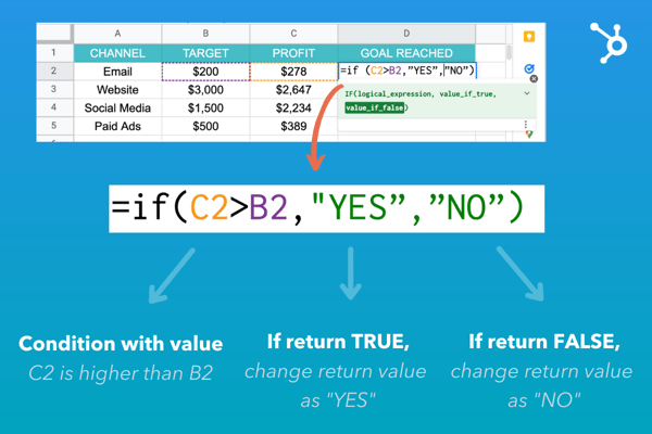
Here, we have a spreadsheet with data on how each marketing channel performed. Each channel had a target revenue next to the actual profit. The last column, “goal reached” will be used to quickly answer which channels met the goal.
-
Select the cell in which the formula will be applied.
-
Write out the formula following this syntax:

-
Drag the mouse to apply the formula to relevant cells.
Scared you’ll forget it? Don’t worry. Google Sheets has an autofill feature that will show you the formula as you type it out.

In this case, the formula will be: =if (C2 > B2, “YES” , “NO”). To break that down further, the formula states if the profit from the email channel is higher than the targeted profit, then write “YES.” If it’s lower, then write “NO.”

Keep in mind that the value if true can be whatever you choose. However, in this example, the simple option was choosing the words “YES” or “NO.”
Because the formula includes words, you must use apostrophes so that Google Sheets reads the formula correctly.
If/Then vs. If/And vs. If/Or Functions
In the simplest terms, with “If-Then” you’re checking that one condition is met. In the example above, it was that one value would be higher than the other. Based on that data, the return value would be “YES” or “NO.”
With “If And,” you’re checking multiple conditions for a “TRUE” value. They all have to be “TRUE” for the return value to be “TRUE.”
“If Or” is the exact opposite to “If and.” It also checks multiple conditions but if any one is true, it will return a “TRUE” value.
Here’s a real-world example:
- If then – I am going to the store. If you go to the store, the statement is true.
- If and – I am going to the store and filling up my tank. You must go to the store and fill up your tank for the statement to be true. Otherwise, it will be false.
- If or – I am going to the store and filling up my tank. You could complete either task and the statement will be true. The only time it will be false if you complete neither one.
How to Use If Function with Multiple Conditions
Say you’re running a survey and you want to easily categorize your respondents into two age buckets. You could write a formula that states if respondents are 25 or younger, they’ll be in group “A”. If they’re 26 or older, they’ll be in group B.
This creates multiple conditions under which the value can be written. The formula checks the first condition, if it doesn’t apply, it moves on to the next to find the appropriate value.
Let’s see this in action.

Using the example above, your formula would be as follows:
= IF(A2 < = 25, “A”, IF(A2 >= 25, “B”))

Nested If Function in Google Sheets
In Google Sheets, “nesting” simply refers to placing the “if” function within its own formula to test multiple conditions and return different results based on those tests.
The formula syntax is as follows:
=IF(first_statement,value_if_true,IF(second_statement,value_if_true,value_if_false))
It’s as easy as that.
So, here’s another function you can use to speed up your process when using Google Sheets.
![]()

![→ Access Now: Google Sheets Templates [Free Kit]](https://no-cache.hubspot.com/cta/default/53/e7cd3f82-cab9-4017-b019-ee3fc550e0b5.png)

